In [1]:

#티스토리 윈도우 사이즈 맞추기
from IPython.core.display import display, HTML
display(HTML("<style>.container { width:90% !important; }</style>"))

In [2]:

import scipy as sp
import numpy as np
import pandas as pd
from scipy import stats

In [3]:

cpi_korea = pd.read_csv("소비자물가지수_2020100__20230107180655.csv", encoding='cp949')

In [4]:

cpi_korea.info()

<class 'pandas.core.frame.DataFrame'>
RangeIndex: 19 entries, 0 to 18
Data columns (total 2 columns):
 #   Column  Non-Null Count  Dtype  
---  ------  --------------  -----  
 0   시점      19 non-null     int64  
 1   전국      19 non-null     float64
dtypes: float64(1), int64(1)
memory usage: 432.0 bytes

In [5]:

cpi_korea['시점'] = cpi_korea['시점'].astype(str)

In [6]:

cpi_korea['시점'] = pd.to_datetime(cpi_korea['시점'], format='%Y')

In [7]:

cpi_korea['시점']

Out[7]:

0    2004-01-01
1    2005-01-01
2    2006-01-01
3    2007-01-01
4    2008-01-01
5    2009-01-01
6    2010-01-01
7    2011-01-01
8    2012-01-01
9    2013-01-01
10   2014-01-01
11   2015-01-01
12   2016-01-01
13   2017-01-01
14   2018-01-01
15   2019-01-01
16   2020-01-01
17   2021-01-01
18   2022-01-01
Name: 시점, dtype: datetime64[ns]

In [8]:

cpi_korea.head()

Out[8]:

	시점	전국
0	2004-01-01	72.418
1	2005-01-01	74.413
2	2006-01-01	76.081
3	2007-01-01	78.010
4	2008-01-01	81.656

In [9]:

import datetime as dt

In [10]:

index = pd.date_range(start='2003-01-01', end='2022-01-01', freq='AS')
index

Out[10]:

DatetimeIndex(['2003-01-01', '2004-01-01', '2005-01-01', '2006-01-01',
               '2007-01-01', '2008-01-01', '2009-01-01', '2010-01-01',
               '2011-01-01', '2012-01-01', '2013-01-01', '2014-01-01',
               '2015-01-01', '2016-01-01', '2017-01-01', '2018-01-01',
               '2019-01-01', '2020-01-01', '2021-01-01', '2022-01-01'],
              dtype='datetime64[ns]', freq='AS-JAN')

In [11]:

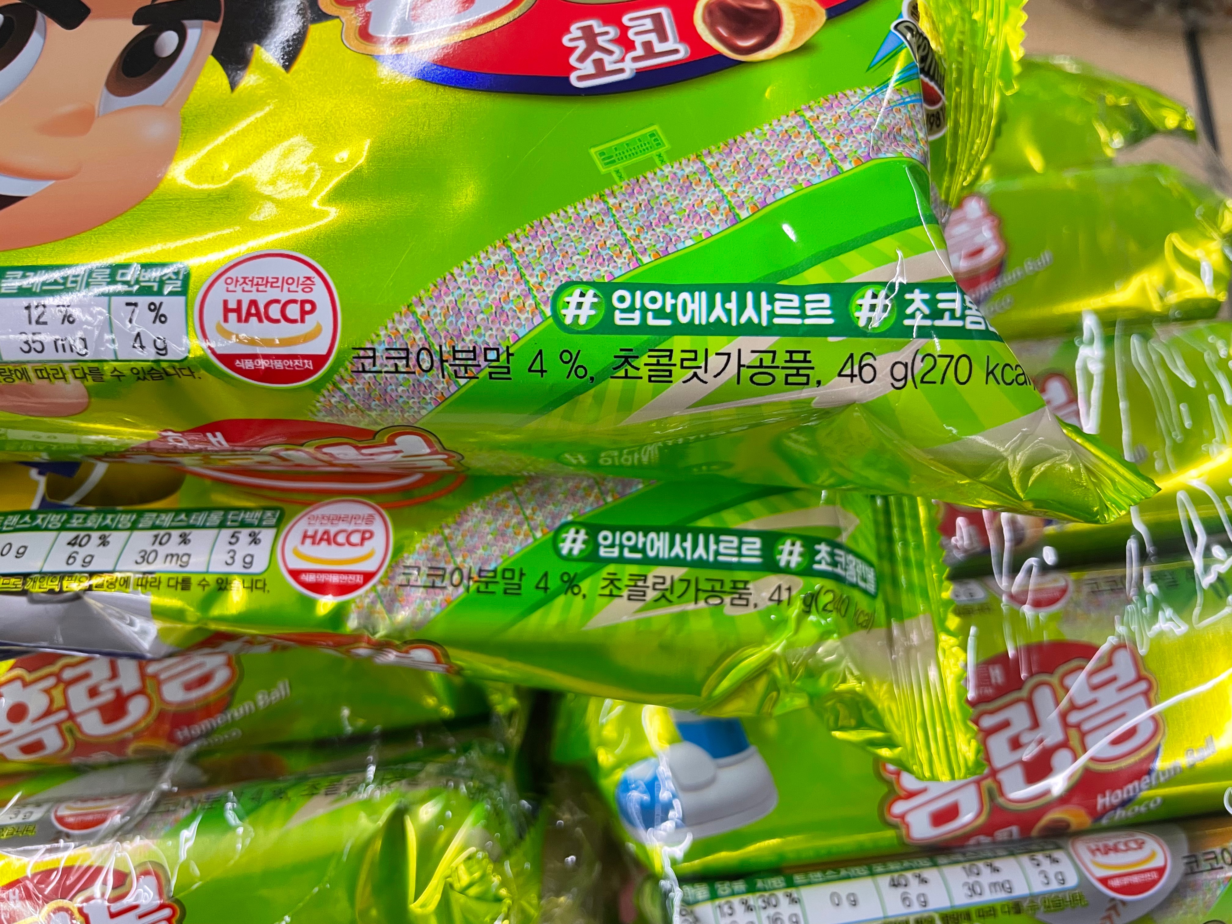
data = {'가격':[440, 700, 700, 1000, 1000, 1200, 1200, 1200, 1200, 1400, 1400, 1500, 1500, 1500, 1500, 1500, 1500, 1500, 1700, 1700],
        '중량':[55, 51, 51, 51, 51, 46, 46, 46, 46, 46, 46, 46, 46, 46, 46, 46, 46, 41, 41, 41]}
index = pd.date_range(start='2004-01-01', end='2023-01-01', freq='AS')
homerun_ball = pd.DataFrame(data, index = index, columns=['가격','중량'])

# 2004년 440원 / 55g => 2023년 1700원 / 41g

# 2004년 가격인상 +260원, 중량절감 -4g
# 2006년 가격인상 +300원
# 2008년 가격인상 +200원, 중량절감 -5g
# 20011년 가격인상 +200원
# 2013년 가격인상 +100원
# 2019년                  중량절감 -5g
# 2021년 가격인상 +200원

In [12]:

homerun_ball['1g당_가격'] = round(homerun_ball['가격'] / homerun_ball['중량'], 0)
homerun_ball

Out[12]:

	가격	중량	1g당_가격
2004-01-01	440	55	8.0
2005-01-01	700	51	14.0
2006-01-01	700	51	14.0
2007-01-01	1000	51	20.0
2008-01-01	1000	51	20.0
2009-01-01	1200	46	26.0
2010-01-01	1200	46	26.0
2011-01-01	1200	46	26.0
2012-01-01	1200	46	26.0
2013-01-01	1400	46	30.0
2014-01-01	1400	46	30.0
2015-01-01	1500	46	33.0
2016-01-01	1500	46	33.0
2017-01-01	1500	46	33.0
2018-01-01	1500	46	33.0
2019-01-01	1500	46	33.0
2020-01-01	1500	46	33.0
2021-01-01	1500	41	37.0
2022-01-01	1700	41	41.0
2023-01-01	1700	41	41.0

In [13]:

homerun_ball['시점'] = homerun_ball.index

In [14]:

homerun_ball.info()

<class 'pandas.core.frame.DataFrame'>
DatetimeIndex: 20 entries, 2004-01-01 to 2023-01-01
Freq: AS-JAN
Data columns (total 4 columns):
 #   Column  Non-Null Count  Dtype         
---  ------  --------------  -----         
 0   가격      20 non-null     int64         
 1   중량      20 non-null     int64         
 2   1g당_가격  20 non-null     float64       
 3   시점      20 non-null     datetime64[ns]
dtypes: datetime64[ns](1), float64(1), int64(2)
memory usage: 800.0 bytes

In [15]:

homerun_ball['가격']

Out[15]:

2004-01-01     440
2005-01-01     700
2006-01-01     700
2007-01-01    1000
2008-01-01    1000
2009-01-01    1200
2010-01-01    1200
2011-01-01    1200
2012-01-01    1200
2013-01-01    1400
2014-01-01    1400
2015-01-01    1500
2016-01-01    1500
2017-01-01    1500
2018-01-01    1500
2019-01-01    1500
2020-01-01    1500
2021-01-01    1500
2022-01-01    1700
2023-01-01    1700
Freq: AS-JAN, Name: 가격, dtype: int64

In [16]:

df_merged = pd.merge_asof(cpi_korea, homerun_ball )

In [17]:

df_merged.columns = ['시점','CPI','가격','중량','1g당_가격']

In [18]:

import matplotlib.pyplot as plt

plt.rc('font', family='NanumGothic')
plt.figure(figsize=(20, 8))

# 데이터
y1_value = df_merged['중량']
y2_value = df_merged['가격']
y3_value = df_merged['1g당_가격']
y4_value = df_merged['CPI']

plt.subplot(1, 2, 1)
plt.title('\n 2004~2022 홈런볼 중량 및 가격 변화 \n', fontsize=20, font="NanumGothic")

# 바차트 : YoY
bar = plt.bar(df_merged['시점'], y1_value, align='center',hatch="//",
                 edgecolor = 'yellow', label='중량', width=200, color='yellowgreen') 

plt.xlabel('DATE')
plt.ylabel('중량')
plt.grid()
plt.ylim(0,60)
plt.legend(loc=2)

plt.twinx()
plt.plot(df_merged['시점'], y2_value, color='green', label='가격',marker='v')
plt.ylabel('가격')

plt.legend(loc=1)
plt.ylim(0,1800)

###
ax1 = plt.subplot(1, 2, 2)
plt.title('\n 2004~2022 홈런볼 1g 당 가격변화(정규화 전) \n', fontsize=20, font="NanumGothic")

ax1.plot(df_merged['시점'], y3_value, color='midnightblue', marker='*', label='1g당 가격')
ax1.set_ylabel('홈런볼 1g당 가격')
ax1.legend(loc=2)


ax2 = ax1.twinx()
ax2.plot(df_merged['시점'], y4_value, color='red', marker='*', label='소비자물가지수')#, secondary_y=True)

ax2.set_ylabel('한국 소비자물가지수')
ax2.legend(loc=1)
plt.grid()

plt.show()

In [19]:

df_merged

Out[19]:

	시점	CPI	가격	중량	1g당_가격
0	2004-01-01	72.418	440	55	8.0
1	2005-01-01	74.413	700	51	14.0
2	2006-01-01	76.081	700	51	14.0
3	2007-01-01	78.010	1000	51	20.0
4	2008-01-01	81.656	1000	51	20.0
5	2009-01-01	83.906	1200	46	26.0
6	2010-01-01	86.373	1200	46	26.0
7	2011-01-01	89.850	1200	46	26.0
8	2012-01-01	91.815	1200	46	26.0
9	2013-01-01	93.010	1400	46	30.0
10	2014-01-01	94.196	1400	46	30.0
11	2015-01-01	94.861	1500	46	33.0
12	2016-01-01	95.783	1500	46	33.0
13	2017-01-01	97.645	1500	46	33.0
14	2018-01-01	99.086	1500	46	33.0
15	2019-01-01	99.466	1500	46	33.0
16	2020-01-01	100.000	1500	46	33.0
17	2021-01-01	102.500	1500	41	37.0
18	2022-01-01	107.710	1700	41	41.0

In [20]:

(107.7 - 72.4)/72.4

Out[20]:

0.4875690607734806

In [21]:

107.7/72.4

Out[21]:

1.4875690607734806

In [22]:

(41-8)/8

Out[22]:

4.125

In [23]:

41/8

Out[23]:

5.125

서로 다른 스케일의 두 데이터를 정규화¶

In [24]:

# 2017.7 = 100 기준인 US값을 400.67 로 나눠주고 100을 곱해 환산해줍니다.
df_merged_new = df_merged[['시점']].copy()

base_point_CPI = float(df_merged['CPI'][df_merged['시점']=='2004-01-01'])
base_point_HRB = float(df_merged['1g당_가격'][df_merged['시점']=='2004-01-01'])

df_merged_new['CPI(2004=100)'] = df_merged['CPI'] / base_point_CPI * 100
df_merged_new['HRB(2004=100)'] = df_merged['1g당_가격'] / base_point_HRB * 100

In [25]:

df_merged_new

Out[25]:

	시점	CPI(2004=100)	HRB(2004=100)
0	2004-01-01	100.000000	100.0
1	2005-01-01	102.754840	175.0
2	2006-01-01	105.058135	175.0
3	2007-01-01	107.721837	250.0
4	2008-01-01	112.756497	250.0
5	2009-01-01	115.863459	325.0
6	2010-01-01	119.270071	325.0
7	2011-01-01	124.071363	325.0
8	2012-01-01	126.784777	325.0
9	2013-01-01	128.434919	375.0
10	2014-01-01	130.072634	375.0
11	2015-01-01	130.990914	412.5
12	2016-01-01	132.264078	412.5
13	2017-01-01	134.835262	412.5
14	2018-01-01	136.825099	412.5
15	2019-01-01	137.349830	412.5
16	2020-01-01	138.087216	412.5
17	2021-01-01	141.539396	462.5
18	2022-01-01	148.733740	512.5

In [26]:

import matplotlib.pyplot as plt

plt.rc('font', family='NanumGothic')
plt.figure(figsize=(20, 8))

# 데이터
y1_value = df_merged['중량']
y2_value = df_merged['가격']
y3_value = df_merged_new['CPI(2004=100)']
y4_value = df_merged_new['HRB(2004=100)']

plt.subplot(1, 2, 1)
plt.title('\n 2004~2022 홈런볼 중량 및 가격 변화 \n', fontsize=20, font="NanumGothic")

# 바차트 : YoY
bar = plt.bar(df_merged['시점'], y1_value, align='center',hatch="//",
                 edgecolor = 'yellow', label='중량', width=200, color='yellowgreen') 

plt.xlabel('DATE')
plt.ylabel('중량')
plt.grid()
plt.ylim(0,60)
# plt.margins(x=0)
plt.legend(loc=2)

# for rect in bar:
#     height = rect.get_height()
#     plt.text(rect.get_x() + rect.get_width()/2.0, height-5, '%.1f g'% height, ha='center', va = 'bottom', size=12, color='red')

plt.twinx()
plt.plot(df_merged['시점'], y2_value, color='green', label='가격',marker='v')
plt.ylabel('가격')

plt.legend(loc=1)
plt.ylim(0,1800)

###

ax1 = plt.subplot(1, 2, 2)
plt.title('\n 2004~2022 홈런볼 가격(1g) vs. 소비자물가지수 \n', fontsize=20, font="NanumGothic")

# fig, ax1 = plt.subplots()
ax1.plot(df_merged['시점'], y3_value, color='midnightblue', marker='*', label='홈런볼 가격지수')
ax1.set_ylabel('홈런볼 1g당 가격')
ax1.legend(loc=2)
ax1.set_ylim(0,600)

ax2 = ax1.twinx()
ax2.plot(df_merged['시점'], y4_value, color='red', marker='*', label='소비자물가지수')#, secondary_y=True)

ax2.set_ylabel('한국 소비자물가지수')
ax2.set_ylim(0,600)

# for i in range(len(xtick_label_position)):
#     height = homerun_ball['1g당_가격'][i]
#     plt.text(homerun_ball['시점'][i], height-1, '%d원/g'% height, ha='center', va = 'bottom', size=10)
ax2.legend(loc=1)
plt.grid()

plt.show()

In [27]:

# 1. 기본 스타일 설정
plt.rc('font', family='NanumGothic')
plt.rcParams['figure.figsize'] = (20, 8)

# 2. 데이터 준비
x = df_merged_new['시점']
y1 = df_merged_new['CPI(2004=100)']
y2 = df_merged_new['HRB(2004=100)']

# 3. 그래프 그리기
fig, ax1 = plt.subplots()

# y1 
ax1.plot(x, y1, '-s', color='green', markersize=3, linewidth=3, alpha=0.7, label='대한민국 소비자 물가지수')

# y2 
ax1.plot(x, y2, '-s', color='blue', markersize=3, linewidth=3, alpha=0.7, label='1g당 홈런볼 가격')

ax1.set_xlabel('DATE')
ax1.set_ylabel('INDEX')
ax1.tick_params(axis='both', direction='in')


ax1.set_zorder(ax2.get_zorder() + 10)
ax1.patch.set_visible(False)
ax1.legend(loc='upper left')

plt.show()

'빅데이터(Big Data) 이론과 코드 > 6. 통계지식' 카테고리의 다른 글

최대 우도 추정법(Maximum Likelihood Estimation, MLE) (0)	2025.01.06
예산과 전문가 없이 데이터로 인포그래픽을 만들기 (1)	2024.06.25
마트 홈런볼과 편의점 홈런볼의 독립표본 t검정 (1)	2023.01.18
[홈런볼로 배우는 데이터 경제] t검정 (1)	2022.12.26
왜도(skewness)와 첨도(kurtosis) (0)	2022.02.28

데이터는 모두에게 동등한 기회를 제공하는가?

홈런볼 슈링크플레이션과 소비자 물가지수

서로 다른 스케일의 두 데이터를 정규화¶

'빅데이터(Big Data) 이론과 코드 > 6. 통계지식' 카테고리의 다른 글

티스토리툴바

홈런볼 슈링크플레이션과 소비자 물가지수

서로 다른 스케일의 두 데이터를 정규화¶

'빅데이터(Big Data) 이론과 코드 > 6. 통계지식' 카테고리의 다른 글

'빅데이터(Big Data) 이론과 코드/6. 통계지식' Related Articles

티스토리툴바